Artist2Vec: Learning Vector Representations of Artists
Let’s learn vector representations of music artists using a corpus of Spotify playlists, and discover some good music in the process!
Try it out - enter an artist or band you love!
Introduction
I love music and I love data science. And I love to use existing things in unexpected ways.
So when I had to come up with a project idea in a course on “Machine Learning for Natural Language processing”, I decided to train a Word2Vec model on an unexpected dataset - Spotify playlists!
Many moons later (about 5 years, so over 1800 of them!), I decided to redo this project, write about it, and hopefully help you discover some good music!
Rationale
My thought process was roughly the following:
- Word2Vec makes use of the linguistic principle called the “distributional hypothesis”, which states that words which occur in similar contexts tend to have similar meanings. (Harris, 1954)
For now, let’s think of “occur in similar context” as words co-occuring in sentences. - Word2Vec models are trained on text, i.e. sentences with words (bare with me).
- Abstracting away from this, we can train a Word2Vec model on anything, as long as we have something like sentences and something like words.
- Spotify users group similar music into playlists, which are available as datasets.
- We can view playlists as something like sentences where the artists become something like words.
- If we train a Word2Vec model on this data, the result will give us vector representations of artists which we can use for music recommendation!
Obviously, this will not be the best music recommendation system ever (I recommend Music-Map for finding music!), I rather created it to prove a point. (And because I needed something fun to program).
Word2Vec
Word2Vec was introduced in 2013 by the paper “Efficient Estimation of Word Representations in Vector Space”, the first author being Tomáš Mikolov1 (at the time at Google). While not the first word embedding model making use of neural networks (see Bengio et al., 2003), Word2Vec was a a much simpler and more efficiently trainable model, especially with the addition of Negative Sampling, introduced shortly after by the same authors. Word2Vec quickly became very influential and garnered a lot of attention of NLP practitioners as it allowed training with far bigger corpora and because neural network language models reduced the need for preprocessing.
Graphical explanation (simplified)
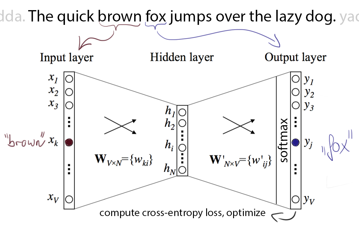
Word2Vec can be concisely explained by looking at an example graphic. Imagine we have a large text corpus and we iterate over every word in this corpus one by one. We also have a simple neural network that will try to learn, given the current word, to predict the next word.
 |
|---|
| Source: own, heavily adapted from ”Word2Vec Parameter Learning Explained“ by Rong |
In the figure above, we are currently at one occurrence of the word ”brown“ in our corpus. We feed it into the pictured simple neural network models one-hot encoded input layer. Then, the network computes the hidden layer as \(h = i^TW\) . Notice that, as the input vector \(i\) is one-hot encoded, this essentially only selects one row from the matrix \(W\), which contains all word representations. No non-linearity is applied in the hidden layer. The hidden layer then gets multiplied by the matrix \(W'\) (notice the prime), which also contains word vectors for every word. This matrix is generally distinct from \(W\) but it is only there to make the math a bit easier, in the end one can freely choose from which matrix to extract the representations. The output of this multiplication, \(o_{pre} = hW'\), is then fed through the softmax non-linearity to get the final output layer \(o_{soft}\) , which, like the input layer, has one entry per word in the vocabulary. The model is now trained to output large values for more probable next words and small values for less probable words. This is done by using our knowledge about what word follows (“fox”, in this case) to compute and minimize the cross-entropy loss by optimizing the variables in our model, namely \(W\) and \(W'\).
Details: Computational considerations
For growing \(V\) (vocabulary size) or \(N\) (vector dimension), training using cross entropy gets intractable rather quickly. Firstly, the second matrix product will become slow, but even worse, the computation of the softmax requires taking \(V\) exponentials and dividing every one of those by their sum. In the original paper, the authors argue that using a hierarchical softmax representation for the output layer can alleviate this burden on the model. This method works by representing the vocabulary in an optimal Huffman binary tree and reducing the output layers to less than \(log_2(V)\) entries, which then assign relative probabilities of the child nodes, essentially defining a random walk that assigns probabilities to words. This method was already proposed in by Bengio et al..
Details: Skip-Gram and Continuous Bag Of Words
The figure above was for illustration purposes only. The paper actually introduced two models, both similar to the one shown above, that either make the model predict the middle word from multiple context words (”CBOW“), or make it predict multiple context words from one middle (or ”target“) word:
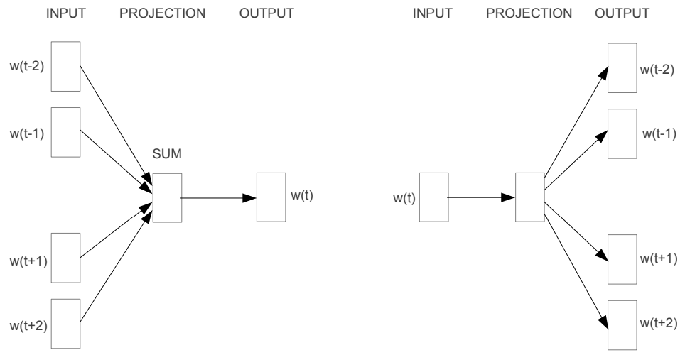 The figure above shows CBOW and Skip-Gram models, respectively. Source: Mikolov, 2013
Sidenote: Other word embedding methods?
You may ask: why not use some other (read: more fancy) word embedding methods? Sure, I could have used, e.g. GloVe, another popular word embedding method that performs dimensionality reduction on the word-context co-occurrence matrix. But constructing the word-word co-occurence matrix seemed infeasible considering the amount of words I have. Also, I was already familiar with Word2Vec and also its GenSim implementation seemed higher quality than what I found for GloVe when looking online. Other word embedding methods, e.g. W2G, W2GM, FastText and ProbabilisticFastText add various bells and whistles, but these are not needed or even counterproductive. The latter two methods subdivide words into word-parts and learn representations for those, and all of the listed methods try to model multiple word-meanings, which would only make sense for artists who release very heterogeneous music. IMHO, it was simply not worth the hassle and the considerable loss in training speed!
Spotify playlists dataset
The dataset I used is provided by Spotify itself and was released in 2020. It features about 2 million unique tracks across exactly 1 million playlists, featuring covering about 300 thousand unique artists in total.
Each entry of the dataset is a playlist, providing metadata on the playlist itself (name, number of followers, total duration, etc) as well as on the tracks within it (track name, position in playlist, artist name, album name, duration, etc).
Expand to see an excerpt of the dataset
"playlists": [
        {
            "name": "Throwbacks",
            "collaborative": "false",
            "pid": 0,
            "modified_at": 1493424000,
            "num_tracks": 52,
            "num_albums": 47,
            "num_followers": 1,
            "tracks": [
                {
                    "pos": 0,
                    "artist_name": "Missy Elliott",
                    "track_uri": "spotify:track:0UaMYEvWZi0ZqiDOoHU3YI",
                    "artist_uri": "spotify:artist:2wIVse2owClT7go1WT98tk",
                    "track_name": "Lose Control (feat. Ciara & Fat Man Scoop)",
                    "album_uri": "spotify:album:6vV5UrXcfyQD1wu4Qo2I9K",
                    "duration_ms": 226863,
                    "album_name": "The Cookbook"
                },
                {
                    "pos": 1,
                    "artist_name": "Britney Spears",
                    "track_uri": "spotify:track:6I9VzXrHxO9rA9A5euc8Ak",
                    "artist_uri": "spotify:artist:26dSoYclwsYLMAKD3tpOr4",
                    "track_name": "Toxic",
                    "album_uri": "spotify:album:0z7pVBGOD7HCIB7S8eLkLI",
                    "duration_ms": 198800,
                    "album_name": "In The Zone"
                },
                ... (49 more tracks hidden)
                {
                    "pos": 51,
                    "artist_name": "Boys Like Girls",
                    "track_uri": "spotify:track:6GIrIt2M39wEGwjCQjGChX",
                    "artist_uri": "spotify:artist:0vWCyXMrrvMlCcepuOJaGI",
                    "track_name": "The Great Escape",
                    "album_uri": "spotify:album:4WqgusSAgXkrjbXzqdBY68",
                    "duration_ms": 206520,
                    "album_name": "Boys Like Girls"
                }
            ],
            "num_edits": 6,
            "duration_ms": 11532414,
            "num_artists": 37
        },
        ... (999.999 more playlists hidden)
]
Dataset analysis
Of course, I started off with some crude dataset analysis.
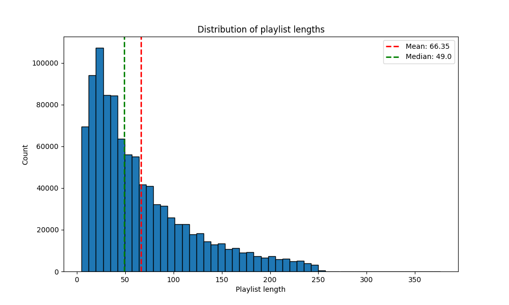
Playlist length
Most popular artists:
Note that this counts artists multiple times if they occur multiple times in a playlist.
| Artist Name | Total Mentions |
|---|---|
| Drake | 847,160 |
| Kanye West | 413,297 |
| Kendrick Lamar | 353,624 |
| Rihanna | 339,570 |
| The Weeknd | 316,603 |
| Eminem | 294,667 |
| Ed Sheeran | 272,116 |
| Future | 250,734 |
| Justin Bieber | 243,119 |
| J. Cole | 241,560 |
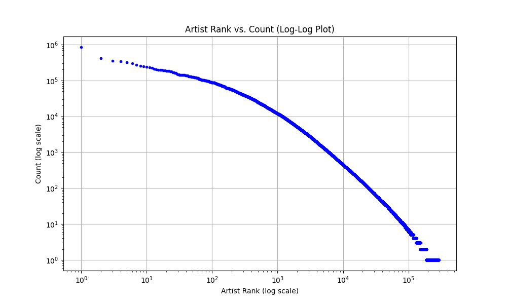
Plotting the rank of the artist against their counts on a log-log scale, we can see Zipf’s law at work:
Learning the vector representations using GenSim
To train the artist vectors, I used the GenSim library.
Preprocessing the data
I pre-processed the data by reducing the playlists to simple lists of artist names. I did not utilize the playlist name nor any other information such as song titles.
Word2Vec first builds a vocabulary by splitting the text on whitespaces. To handle artists with whitespaces in their name, I thus had to remove whitespaces completely before the preprocessing, i.e. “Rage Against the Machine” becomes “RageAgainstTheMachine”.
Running the training
We construct the model and call the training function on it:
model = gensim.models.Word2Vec(playlists, sorted_vocab=1, vector_size=100, window=150, negative=100, workers=8)
model.train(playlists, total_examples=model.corpus_count, epochs=50)
Hyperparameter explanation:
vector_size=100: The dimension of the resulting artist vectors.
window=150: The number of ‘words’ (read: artists) around the current word that count as “context”.
negative=100: During training, a number of negative (unrelated) words/artists are sampled.
epochs=50: The number of epochs (passes through the playlist dataset).
Here is the GenSim.Word2Vec documentation if you’re interested about all the possibilities. Training took about half an hour on a fairly beefy desktop tower.
Other hyperparameters
Fore the sake of completeness: there are two more hyperparameters:
shrink_windows=True: In each training step, the used window size is randomly sampled from [1,window], and thus the algorithm favors closer words. Enabling this helps performance. I suspect artists are indeed more similar the closer they appear in a playlist, but its not a super strong effect.
ns_exponent=0.75: This paper found that for recommendation use cases, a -0.5 is an appropriate value, “such that the negative sampling distribution is more likely to sample unpopular items as negative examples”. However, after trying that, it hurt performance somewhat, so I just left it at the default of +0.75.
Evaluation and hyperparameter search
We skipped a step here - how did I choose those hyperparameters?
Evaluating artist recommendations using Spotify API
From the start of this project, one thought kept nagging me: how to evaluate this? In normal Word2Vec models, you can for example correlate some word-word similarity scores to human-rated similarities from some dataset, e.g. WordSim353. However, we don’t really have a ground truth dataset for artist similarities expressed as scalar values. 🤔
But then, while browsing the documentation of the Spotify Web API, I stumbled across this: /artists/{id}/related-artists. This API endpoint gives us 20 related artists, but no scalar value how similar they are to the provided artist. While that doesn’t allow me to directly correlate similarity scores, I can still use it and compute the average number of matches between the twenty top related artists (as computed by the trained model) and the data i get from the Web API, across a larger number of artists.
When computing these scores for some models I trained, I noticed that some hyperparameter settings work really well for popular artists (say, from the top-1000) but perform much worse for less popular artists (say, from rank 10000 and up) and vice-versa. I decided to crawl the related artists for three “popularity groups”: top (the top 1,000 artists), mid (1,000 randomly sampled artists from ranks 1,000 to 10,000) and low (1,000 randomly sampled artists from ranks 10,000 and up) and compute the metric for all of them separately to get a more fine-grained evaluation.
Hyperparameter search
Equipped with an evaluation function, I started to produce some plots for selecting the various hyperparameters.
Selecting the number of epochs and negative samples:
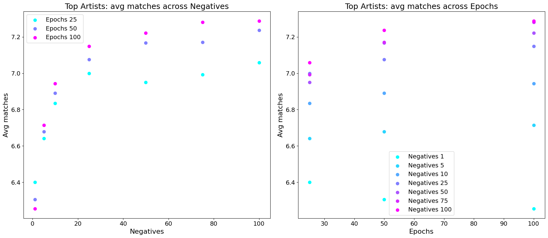
Arbitrarily fixing the vector Size to 100 and the window size to 150 for now, I plotted the effect of the hyperparameters “negatives” and “epochs”:
First, a plot when evaluating using the “top” artists only:
Now, let’s look at the performance on “low” artists:
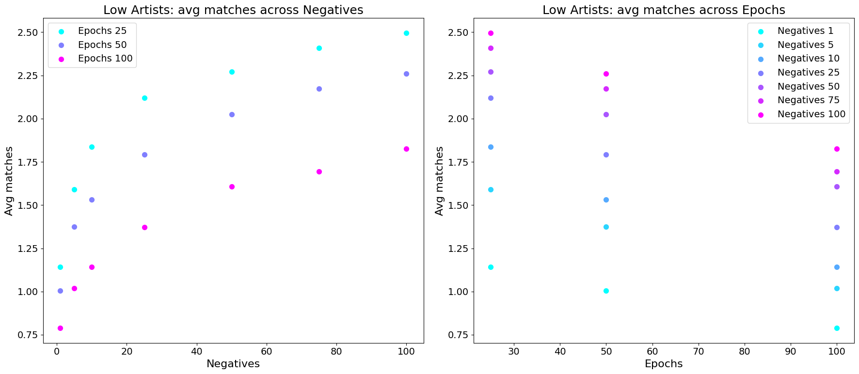
So, it seems that more negative samples helps in both cases, but increasing the epochs hurts the performance for less popular artists.
We can also produce an averaged performance plot across all three popularity groups:
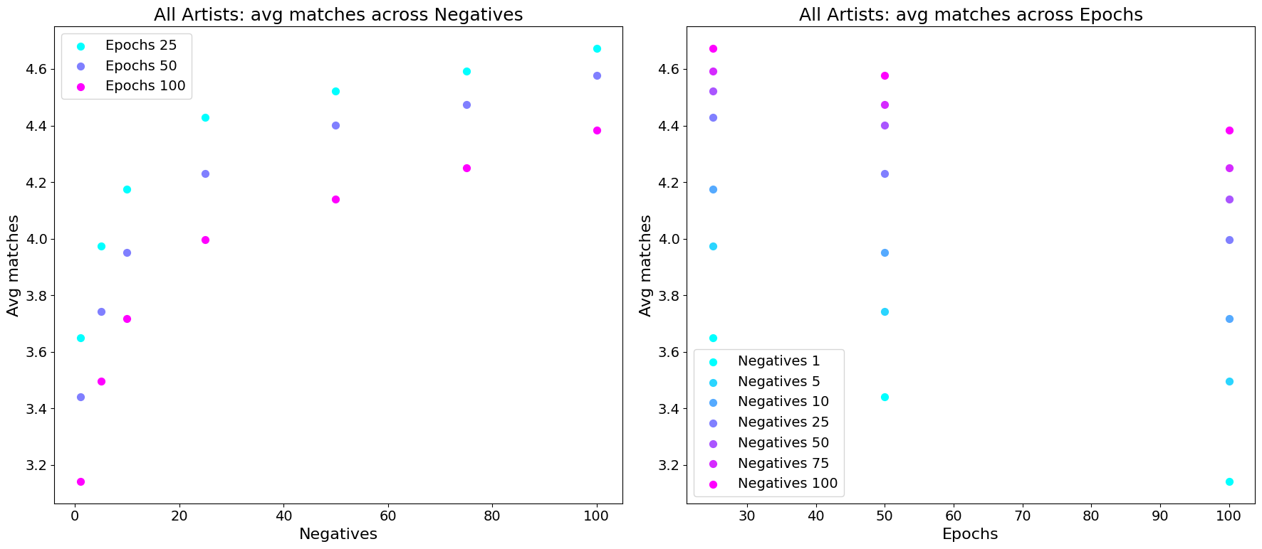
From these plots, I decided to go for 100 negative samples and 50 epochs for a reasonable trade-off in performance across the groups.
Selecting the vector size and window size:
Next I produced similar plots for the other two hyperparameters, while keeping negatives set to 100 and training for 50 epochs:
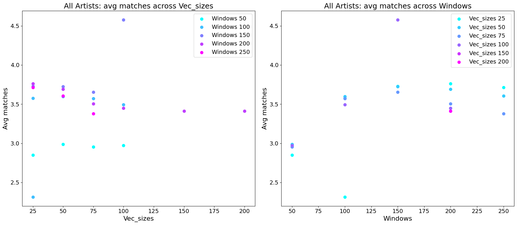
Looking at it, it seems clear that a vector size of 100 and a window size of 150 is optimal. But this should make us pause - these are exactly the hyperparameter values we arbitrarily chose in the beginning! I don’t think this is a coincidence - in the previous step we CHOSE the 100 negative samples and 50 epochs because they worked best with these two hyperparameter values - and now it turns out no other values can perform equally as good paired with them. But, and I have no data to back this up, but I am pretty sure similar performance can be reached with other hyperparameters if we started out with a different initial hyperparameter choice. For now, let’s settle for this set of hyperparameters.
A detour about co-evolution of some NN architectures and optimizers
This reminds me of something, and I want to take this opportunity to share this blogpost, which blew my mind the first time I read it. The optimizer Adam, as the ML conventional wisdom rightfully holds, works well across a large variety of proposed neural network architectures found in literature. But the subtle reason that Adam emerged as the go-to optimizer, as purported by the blog post, is that these architectures we are evaluating it on were selected while keeping the optimizer fixed to what was known to work on more basic architectures, e.g. Adam. When we now change Adam to, say, SGD, we converge to a bigger loss, but we probably could have gotten a similarly low loss using an architecture that was selected in architecture search using SGD as the optimizer.
Visualization of learned vectors using UMAP
To visualize the high-dimensional artist vectors, I used the dimensionality reduction technique called “Uniform Manifold Approximation and Projection” (UMAP), as implemented in the umap-learn NodeJS library.
UMAP works by constructing a high-dimensional graph representation of the data and then finding a low-dimensional embedding that preserves the essential topological structure of this graph. In our case, we use UMAP to reduce our 100-dimensional artist vectors to 3 dimensions, which we can then visualize in an interactive 3D scatter plot:
Artist arithmetics
One of the fascinating aspects of Word2Vec is its ability to capture semantic relationships in vector space. A classic example is the analogy “king - man + woman = queen”, where vector arithmetic on word embeddings yields meaningful results.
In the context of our artist vectors, we might hope to find similar relationships. But, pondering this for a bit, I couldn’t come up with a good example set of artists to try this out with. If you have a clever idea about this, please reach out! :-)
Building a webapp from it
Finally, I built the above webapp to share this fun little experiment with the world. (Note: I hacked this together rather quickly.. ‘here be dragons’!)
Webserver using Node.JS+Express+usearch+umap-js
I set up a simple Node.js server using Express to handle API requests. The server loads the artist data vector embeddings (saved from Python as JSON), then uses usearch to build an index for efficient nearest neighbor searches, and computes UMAP embeddings of three components using the umap-js library. The index and embeddings are stored to files and loaded on startup for performance reasons. I added simple rate limiting using the express-rate-limit package to prevent abuse.
When returning nearest artists, the webserver uses the Spotify API to also fetch their profile picture, follower count and genres. It uses a SQLite database to cache all Spotify API queries with unlimited TTL.
Frontend React app
The frontend is simple React applications:
- Artist Search and Recommendation:
- Autocomplete in search inputs done using the simple rule
artist.name.toLowerCase().includes(searchTerm.toLowerCase()) - Fetches the server for recommended artists based on vector similarity
- Shows result artist images, names, genres and the computed distance to the searched artist
- Autocomplete in search inputs done using the simple rule
- 3D Scatter Plot Visualization:
- Loads 3-dimensional embeddings from the server
- Uses ScatterGL to render a 3D visualization of the embeddings
Conclusion
- I explored the application of the Word2Vec method for music artist recommendation
- I treated playlists as sentences and artists as words in these sentences
- Artists get mapped to vectors which can be used to perform vector similarity search
- I added evaluation using the Spotify Web API
- I made a very simple web application to allow you to find good music (hopefully!)
Potential future work:
- Investigating “artist arithmetic” and extracting meaningful directions in embedding space
Thanks for reading!
Personal music recommendations:
Here is some music I love :-)
-
An interesting tidbit from his Wikipedia page: “Mikolov came up with the idea to generate text from neural language models in 2007 and his RNNLM toolkit was the first to demonstrate the capability to train language models on large corpora, resulting in large improvements over the state of the art.” ↩