This post explains the paper “Modality-Agnostic Variational Compression of Implicit Neural Representations”, first-authored by Jonathan Schwarz, a Senior Research Scientist at DeepMind and PhD candidate at University College London.

I also gave a talk on this paper at a reading group, if you prefer slides.

Overview

This paper proposes a compression algorithm that is applicable across a large variety of modalities. To be specific, it can be applied in all cases where the data points can each be represented as a function mapping coordinates to features. These functions can then be represented by neural networks, a technique called Implicit Neural Representations, which the presented paper makes use of. The authors compare their method favorably against a variety of modality-specific and other modality-agnostic compression algorithms.

Why strive for modality-agnostic compression algorithms?

Currently, we use custom compression techniques for each modality: if you want to compress some audio data, you’d probably use MP3 or FLAC. The images your browser loaded to show you this page were compressed with JPEG. If you watch a video on YouTube, it is probably compressed with VP9.

All these algorithms work well, in part because they make use of expert knowledge about the data from the respective modalities. While these tricks/biases help the compression reach impressive ratios of filesize-vs-quality, they limit the transfer of algorithmic ideas between compression algorithms for different modalities. Thus, the authors argue for modality-agnostic compression algorithms.

A refresher on implicit neural representations (INRs)

Implicit Neural Representations are a way to represent data points in terms of a neural network. This is done by interpreting data as functions from coordinates to features, e.g. (x,y) to (r,g,b) for images. Then, we can parameterize these functions with neural networks. Implicit Neural Representations are inherently modality agnostic, since they can always be applied as long as the data can be expressed as functions. Other examples besides images include video data, voxels, or audio data. Even graphs have been shown to be representable in such a way. Notably, textual data and tabular data are exempt from the list of modalities that are supported. In the end, a data point is (implicitly) encoded within the weights of a neural network.

Thus, if we want to use these INRs for compression, we have to ask ourselves on how to store those weights efficiently. In a sense, data-compression becomes model-compression. Some previous work (such as COIN and MSCN) simply casted the weights to 16-bit or perform other simple quantization techniques. But we can do better, and this paper, among else, shows how.

Using implicit neural representations for compression

We will soon get to the juicy parts of the paper. But first, let’s formalize the INR and how to optimize it in a naive way:

An INR is a neural network \(f(\cdot; \theta): \mathcal{C} \rightarrow \mathcal{Y}\), with parameters \(\theta\).
We can optimize it using the mean-squared error: \(min_{\theta} \sum_{j=1}^{M} \Vert f(c_j;\theta)-y_j\Vert_2^2\) . Here, M is the number of coordinates (e.g. for a 8x8 pixel image, this would be 64). \(c_j\) is just a particular coordinate, e.g. a tuple (0,0) for the top-left pixel.

Thus, \(f(c_j;\theta)\) is the models prediction for the value at coordinate \(c_j\) of the particular data point this INR is representing. \(y_j\) is the true value of that data point at that coordinate. We sum up over the squared L2 norm of the differences between predicted and true feature values to get our total loss, which we can then optimize using gradient descent.

Now, you may have already noticed that this is not a very efficient way of doing this: we would be learning one whole neural network per entry in our dataset! But there is a clever way to mitigate this issue: we can assume that all the entries in our dataset share some common characteristics, and model these characteristics in one (bigger) network whose weights are shared across all data points, and then adapting these weights slightly for each particular datapoint, storing only that (smaller) change.

Specializing a shared INR

Assume now we have a shared INR \(f(\cdot, \theta)\), meaning it has one set of parameters \(\theta\) that is shared among all datapoints. Then additionally we have data-item specific parameters \(\phi^i\), one per data-item, which contain information on how to adapt the shared network such that the adapted network represents the i’th data item. Again, the \(\theta\) is much larger than the \(\phi^i\).

Now, the next obvious question is: “how to adapt the shared INR \(f\)?”. This process is also called conditioning or specializing. Obviously, we shouldn’t just store weights and biases of the same shapes in \(\phi^i\) and add them to the weights and biases in \(\theta\) in order to specialize it, as this would not save us any storage. Side note: this can actually be done, but it needs some trickery.

Instead, commonly, layer-wise modulations are used. This means that \(\phi^i\) consists of one vector per layer in the shared INR: \(\phi^i = [s^{(1)},...,s^{(L)}]\), assuming \(f\) has \(L\) layers. These vectors each have as many entries as there are neurons in the respective layer. Then, the mapping that represents one layer in the adapted network looks as follows:

\[\begin{equation} c^{(l-1)} \mapsto h(W^{(l)}c^{(l)} + b^{(l)} + s^{(l)} ) \end{equation}\]

We see that in the non-linear activation function \(h\), we add the stored vectors to the otherwise untouched neural network feed-forward computation. Here, \(W^{(l)}\) and \(b^{(l)}\) are the weights and biases of the (\(l\)‘th layer of the) shared INR with parameters \(\theta\).

Reducing the size of \(\phi^i\) further

Previous work has proposed two ways to decrease the amount of data we need to store in the \(\phi^i\):

Latent modulation: “From data to functa” proposes to not make the modulation vectors \(s^{(l)}\) the entries of the \(\phi^{(i)}\) directly, but to instead predict the \(s = [s^{(1)},...,s^{(L)}]\) from the \(\phi^{(i)}\) using a mapping, in the Functa case a simple linear mapping: \(s = W'\phi+b'\), where the \(W'\) and \(b'\) are shared across all data items, much like the \(\theta\). So far, these mappings have been limited to linear mappings which, as the authors of the presented work argue, have a lack of representational capacity.
Sparsity: We can also prune dimensions in \(\phi^i\) by inducing sparsity, as done in “Meta-Learning Sparse Compression Networks”. This means we do not modulate every neuron of every layer, and thus the \(s^{(l)}\) contain many zeroes, and can be stored more efficiently. But this technique, at least as proposed in the cited work, requires approximate inference, and thus introduces additional complexity and hyperparameters.

Improving implicit neural representations for compression

Now we can finally move to the core of the paper and its contributions. The authors argue that INR-based compression can be improved in a two-fold approach:

Improved conditioning: We try to achieve the best signal reconstruction error with a limit on the number of entries in \(\phi^{(i)}\)
Improved compression: We compress the \(\phi^{(i)}\) in a better way before actually storing/transmitting them

These two are orthogonal algorithmic considerations. While improving the conditioning increases the upper-bound of performance we can hope to achieve after compression of the \(\phi^{(i)}\), improved compression reduces the gap between that upper-bound and the actual final reconstruction performance, as measured in stored bytes vs. reconstruction quality.

Let’s first look at how the authors propose to improve the conditioning. The improved compression will also be explained later.

Improved conditioning: INR specialization through subnetwork selection

As we have just seen, previous methods either propose latent modulation via parametric predictions or sparsity to achieve better reconstructions at equal capacity (i.e. \(dim(\phi^i)\)). The authors aim to combine the positives of both while avoiding their pitfalls. To achieve this, they propose a middle ground, which learns more effectively and efficiently. We will later see an experimental result that showcases this.

The authors propose to do sparsity, but without hard-gating, and they do latent modulations, but their parametric predictions are done in a non-linear way. Let’s look at this in some more detail, starting with the mapping from one layer to the next in the modulated network, similar to what we had before, but with some crucial differences.

We can see that, our non-linearity has changed from the placeholder \(h(\cdot)\) to \(sin(w_0*(\cdot))\), which is simply the one that proved especially good for INRs, as proposed in the paper “Implicit Neural Representations with Periodic Activation Functions” (“SIREN”).

Instead of the \(s^{(l)}\) vectors we saw earlier, now we have one matrix \(G_{low}^{l}\) per layer, but these matrices still come from the \(\phi^i\). And instead of adding something in the non-linearity \(h\), as seen before, we now elementwise-multiply our weight matrix (coming from the global parameter \(\theta\)). If we peek at the second equation in the image above, we see that the \(G_{low}^{l}\) is the result of a sigmoid applied to something (we’ll look at it shortly), thus its values are in \((0,1)\). The authors call these matrices “soft gating masks”, as they select entries in the weight matrix to adjust (value > 0) and by how much their values should be multiplied. The authors call this process “subnetwork selection”, and this part relates to the mentioned sparsity.

Now, lets look at how these \(G_{low}^{l}\) matrices, of which we have one per layer, are computed from the \(\phi^i\), of which we have one per data-item. We see in the second equation (\(G_{low}^{l} = \sigma(U^{(l)} V^{(l)T})\)), that it is the result of a multiplication of two vectors, \(U^{(l)}\) and \(V^{(l)}\) for which we again have one per layer (as seen by the superscript \(l\)). \(U^{(l)}\) and \(V^{(l)}\) both have shape \(m \times d\), with \(d<<m\), and thus \(G_{low}^{l}\) has the same shape as \(W^{l}\), namely \(m \times m\). The \(d<<m\) ensures that the \(G_{low}^{l}\) has low rank. But, while trying to learn how to get the \(G_{low}^{l}\), we have until now just moved the goalpost! LLet’s learn how to get all the vectors \(U^{(l)}\) and \(V^{(l)}\) from the \(\phi^i\).

We now move to the latent modulation aspect of their proposed method for improving the conditioning. Similar to previous techniques, the \(U^{(l)}\) and \(V^{(l)}\) vectors are not directly the entries of the \(\phi^i\), but they are not the result of a simple affine transform either, as was the case in earlier work. Instead, they are the output of a deep residual network with input \(\phi^i\), whose parameters are subsumed under \(\theta\), i.e. the global parameters.

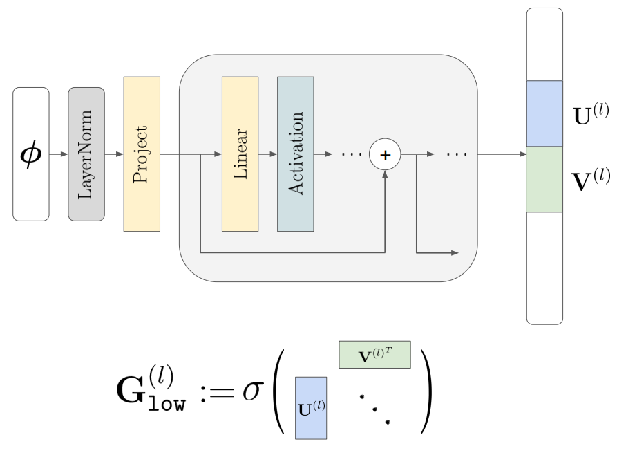
This is Figure 2(a) of the paper. As you can see, we have one network (as opposed to, say, one per layer), that outputs one big vector which is then spliced into all the \(U^{(l)}\) and \(V^{(l)}\) vectors (one each per layer). This network is shallow, consisting of only one or two residual blocks. Details on the architecture hyperparameters can be found on the very last pages of the paper. While previous work found it hard to optimize a non-linear latent prediction network, the authors note that the introduction of the LayerNorm played a major role in making this construction work.

Improved conditioning: How is the whole thing optimized?

Now let’s see how the authors propose to optimize their conditioning system. They make use of an algorithm called “Model-Agnostic Meta Learning” (MAML).

Let’s take a step back first. What parameters are we trying to optimize for?

We need shared INR \(f\) that effectively learns general structure in our data. Its parameters (all weights \(W^{(l)}\) and biases \(b^{(l)}\) in the formulas above) are part of the global parameters, i.e. \(\theta\).
We need to learn the parameters of a deep residual network that maps our \(\phi^i\) to the vectors \(U^{(l)}\) and \(V^{(l)}\). Its parameters are, by definition, also part of \(\theta\).

Now, let’s take a step into the future for a second. Say we had a good shared INR and a good mapping network, and say we freeze them both for now (i.e., we don’t update them in the following). We are now given an unseen image we want to encode, unseen meaning it was not used to fit either of our two networks. We are trying to find a latent modulation vector \(\phi^{(i)}\), that when passed through our mapping network, gives us the \(U^{(l)}\), \(V^{(l)}\) vectors and in turn the \(G_{low}^{l}\) matrices, which when conditioning the shared INR with them, results in an adapted network \(f(\cdot; \theta, \phi^i)\). And of course we want that adapted network to represent our datapoint well, i.e. to reduce the mean-squared error we saw way back when i introduced INRs, let’s denote that error by \(\mathcal{L}({\phi}, x) = \sum_{j=1}^{M} \Vert f(c_j;\theta, \phi)-y_j\Vert_2^2\), here we define \(x = (c,y)\) . I left out the superscripts \(i\) for readability, since it is clear we are searching for a modulation which represents our one particular previously unseen image. To do this, we can start out with a random latent modulation vector \(\phi_0\) and perform a single gradient step, minimizing this loss with respect to the \(\phi_0\), while keeping the \(\theta\) fixed:

\[\phi\star = \phi_{0} - \alpha * \nabla_{\phi_{0}} \mathcal{L}({\phi_{0}},x)\]

Note that the star is a bit misleading, since one iteration of this surely won’t be enough to find a good modulation. Indeed, previous work showed that you have to do upwards of tens of thousands of iterations to converge on a modulation vector with low MSE.

Model-Agnostic Meta Learning (MAML) to the rescue!

The key idea of MAML is to backpropagate through this one-step optimization process I just described. We thus optimize the following objective:

\[\min_{\theta,\phi_0} \mathbb{E}_{x \sim p(x)} [\mathcal{L}(\phi_{0} - \alpha * \nabla_{\phi_{0}} \mathcal{L}({\phi_{0}},x), x)],\]

which is the expected reconstruction quality after being allowed to update the modulation for one step, starting from \(\phi_0\). The idea now is that, beyond the \(\theta\) parameter, we can now additionally learn a good \(\phi_0\) parameter, e.g. a good starting point from which we can find a modulation vector \(\phi^i\). Even more, we can also learn the step-size \(\alpha\), as in “Meta-SGD”. Using these two improvements, previous work has already shown that we can find a reasonably good modulation vector in as little as ten iterations, starting from the learned \(\phi_0\) and doing gradient descent.

One drawback of MAML is that it requires a lot of memory due to second-order gradients being used. This forces the authors to encode data in patches, i.e. they compress 32x32 blocks of pixels and store the final (compressed and quantized) modulation vectors \(\phi^i_{\text{patch p}}\) in a concatenated manner. And while there are first-order methods, previous work found them to severely hinder the performance.

This concludes the description of the improved conditioning mechanism. A look at algorithm 1 in the papers appendix should now also be helpful in understanding this optimization procedure.

Improved compression

Let’s move on to improving the compression of the \(\phi^i\) vectors. The authors propose a learned compressor, meaning it is not a fixed function, but instead learned to compress samples from a distribution in the best possible way. It is optimized with the dataset at hand and can then also be applied to any unseen samples.

The authors adapt the method in “End-to-end optimized image compression” for their needs. This method was devised for image data and does not make use of INRs. It learns to encode images as a code with low rate and good reconstructions after quantization. For this purpose, an encoder and decoder, both CNNs, are optimized, as well as an entropy model which learns a probability distribution over the codes, which is needed in entropy coding to store the information using the fewest bits possible, in expectation.

You might be a little confused now: The authors make use of a method for image data, which does not even make use of INRs? How can they apply this? The answer is that they do not apply this method to the inputs, but to the modulation vectors! And since these are vectors, no matter the initial modality, we keep our treasured modality agnosticism. In the encoder and decoder models, we replace the convolutions by linear layers.

The referenced method works by optimizing a loss comprised of a rate term and a distortion term: \(\begin{align*} \mathcal{L}_{\text{compress}}(\pi_a,\pi_b,x,\phi) &= \mathcal{L}_{\text{ratio}} + \lambda*\mathcal{L}_{\text{distortion}} \\ &= -\text{log}_2[p_{\hat{z}}(Q(g_a(\phi;\pi_a)))] + \lambda*\mathcal{L}_{\text{MSE}}(g_s(\hat z;\pi_s), \phi) \end{align*}\)

Here, \(p_{\hat{z}}\) is the (parameterized) entropy model, Q is a quantizer (which in this case computes the quantized code \(\hat z\) simply as \(\text{round}(z)\)), \(g_a\) and \(g_s\) are the analysis and synthesis transforms, respectively, with \(\pi_a\) and \(\pi_s\) being their parameters. The analysis and synthesis transforms can be thought of as encoder and decoder, the former terms are just the terms used in existing compression literature, where e.g. the analysis transform in JPEG is a DCT and the synthesis transform is the inverse DCT.

We can see that the first term, the rate, is expressed as the entropy, which serves as a proxy to the true rate, read the papers section 3 for more details on this. The second term, the distortion, measures how well we can reconstruct the modulation vector from the quantized z, by applying the synthesis transform and evaluating the MSE to the “true” vector \(\phi\). The two terms are added and the latter is ratioed with the hyperparameter \(\lambda\), which allows to trade-off between getting a small rate or small distortion. Note that for a new hyperparameter \(\lambda\), the whole optimization has to be run anew.

Finally, note that in the end we don’t care about reconstructing the modulation vector \(\phi\) with low distortion, but to reconstruct the image \(x = (c,y)\) that led to the modulation vector. Thus, they replace the distortion loss \(\mathcal{L}_{\text{distortion}}\) by \(\mathcal{L}(f(\cdot; \theta, g_s(\hat z;\pi_s)) ,x)\), noting that this change produced the best reconstructions of the data items.

This concludes the description of the improved compression mechanism. A look at algorithm 2 in the papers appendix should now also be helpful in understanding this optimization procedure, although that one is slightly harder to parse without reading the paper describing the adapted method.

The big picture

Let’s again take a step back to get the bigger picture. We start out with a set of samples from a particular distribution, e.g. a set of images. We use MAML to optimize for the \(\theta\), \(\phi_0\) and \(\alpha\) parameters, as described earlier. We then store these, freeze them, and sweep over the set of samples once more to get one (latent) modulation vector \(\phi^i\) per sample. We take these modulation vectors, and apply the compression method, in turn learning the encoder, decoder and entropy models. Once done, we can compress an unseen sample in the following way: we perform a few iterations from \(\phi_0\) to get a modulation vector \(\phi\), and then pass it through the encoder model and quantizer, and store them using e.g. Huffman coding. To decode it, we undo the Huffman coding, apply the decoder to get our predicted modulation vector back, then we specialize our shared INR \(f\) with it, and evaluate it at all the coordinates to predict the feature values and in turn restore our data point.

Experimental evaluation

With the method explained, we can now take a look at some results. Since the focus of this work is the modality-agnosticism, the authors provide experiments across a variety of modalities.

Effectiveness of advanced conditioning

The first set of experiments is about validation that the improved conditioning is effective. To isolate the effect of the improved conditioning on its own, the authors measure performance across different \(dim(\phi)\), i.e. sizes of the modulation vectors. Let’s have a look at table 1 first. If you’re unfamiliar with any of these datasets, they are explained in Appendix A of the paper.

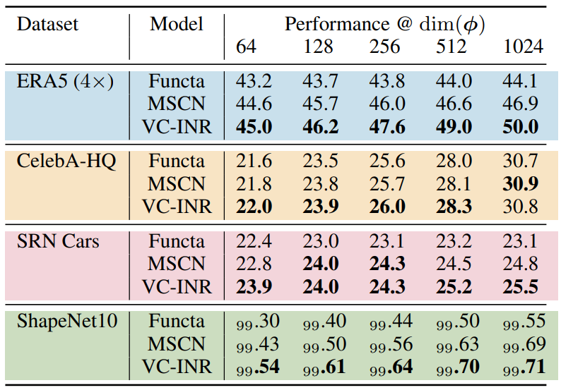
The model is a SIREN with 15 layers of 512 neurons each. The values are the PSNR (\(-10*log_{10}(\text{MSE})\), higher is better) for all but the ShapeNet10 dataset, where it is the Voxel Accuracy. Keep in mind that, since this is a log-scale, the difference between, e.g., Functa on ERA5 at \(dim(\phi)=1024\) where it reached a PSNR of 44.1, and the proposed VC-INR in the same setting, which reached a PSNR of 50.0, is actually quite significant. Overall we can conclude that the proposed mixture of sparsity (as in MSCN) and latent modulation (as in Functa) works consistently better or at least as good as the two ideas on their own.

Effectiveness of non-linearity in the latent modulation

Another ablation the authors did is regarding the effectiveness of the latent modulation prediction network (that maps \(\phi\) to the \(U^{(l)}\) and \(V^{(l)}\) vectors) being non-linear.

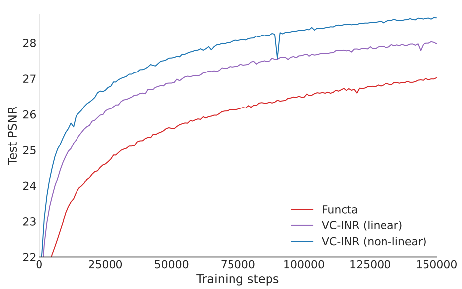
This plot compares the proposed method, “VC-INR (non-linear)”, to a version of VC-INR where the prediction network is just an affine transform, and also comparing against Functa, where we have an affine transform, but the conditioning is different, as explained earlier. The three perform in that order, providing justification for the added complexity introduced by the non-linear latent modulation prediction network.

Effectiveness of advanced compression

Next up, we can look at the performance of the combination of the proposed enhancements. In the following, a dashed line indicates a modality-specific compression algorithm, and these are also denoted with a (s) suffix in the legend. Methods denoted with a (n) suffix are other neural compression methods (note that these can also be either modality-specific or not).

In the following, the Bit-rate (bpp) is defined as \(\frac{\text{number of bits}}{\text{number of pixels}}\), where in non-image data, a “pixel” corresponds to a single dimension of the data. Note that we only count the number of bits we would need to transmit, in particular this does not include the \(\theta\), \(\phi_0\) or \(\alpha\), which we assume are all already distributed to the end users as part of the decompression software.

Modality: Images

In the image modality, we can see that the method outperforms the direct (in that, most comparable) competitors, which are the modality-agnostic neural compression methods COIN and COIN++, and the proposed method also outperforms some modality specific compression methods, including the widely used JPEG. One caveat is that the authors did not give any details on the implementation and configuration of e.g. the JPEG compressor. “Strüpler” should be “Strümpler” and refers to this modality-agnostic method that also meta-learns an initialization, and uses quantization-aware training to compress the modulation vectors.

Modality: Manifold

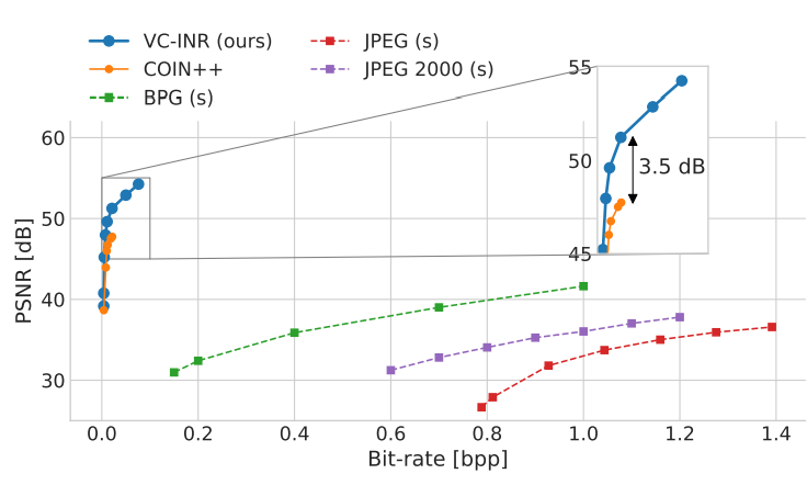
As for manifold data, the authors compress the entries in the ERA5 climate data dataset. The image compression algorithms are applied by unrolling each manifold on a rectangular grid and inputting it as an image. Thus, calling JPEG and its friends “modality-specific” to manifold data is a bit of a stretch here, at least in my opinion. Still, since there is no better alternative around, the comparison does have a raison d’être.

Modality: Audio

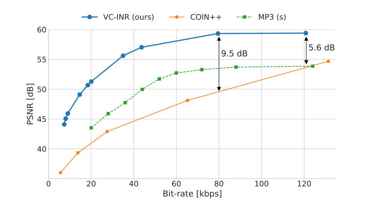
In the audio modality, the LibriSpeech dataset is used, which contains in total 1000 hours of read English speech sampled at 16 kHz. The authors compare against MP3, but again without providing any details on the configuration used. Also, I would have liked to see a comparison with the OPUS codec too, which performs better in general, especially at low bitrates, and especially so in the speech compression setting. My guess is that OPUS would perform best in this low-bitrate speech compression setting.

Modality: Video

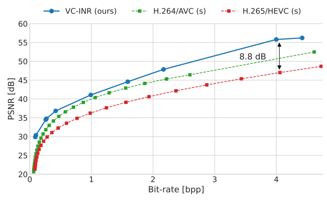
For video, the UCF101 dataset was used, which contains a total of 13320 videos showing a total of 101 human actions such as “knitting”, “basketball” or “golf swing”. It is definitively impressive that the proposed method outperforms a video encoder that is the result of an incredible amount of engineering such as HEVC, although again no details about the configuration are given by the authors.

Conclusion

The authors introduce VC-INR, a modality-agnostic neural compression technique
They argue for modality-agnosticism as a key guiding principle
They propose algorithmic improvements across both conditioning and compression
For improving conditioning, they combine ideas from latent modulation and sparsity
For improving compression, they apply a previous neural compression method to the modulations
The proposed method often even outperforms modality-specific codecs